Belief Propagation
This page describes the concept of belief propagation and message passing
Decoding algorithms for LDPC codes generally derive from the belief propagation (BP) algorithm, which is also termed the sum-product (SP) or message passing (MP) algorithm. The algorithm is a probabilistic algorithm that considers the posterior probabilities of bits ($c_i$) given channel observations $\mathbf{y}$. The algorithm may be phrased in terms of probability:
\[\Pr\left(c_i=1\vert \mathbf{y}\right)\]in terms of likelihood ratio:
\[l(c_i)=\frac{\Pr(c_i=0\vert \mathbf{y})}{\Pr(c_i=1\vert \mathbf{y})}\]or in terms of the log-likelihood ratio:
\[L(c_i)=\log\left(\frac{\Pr(c_i=0\vert \mathbf{y})}{\Pr(c_i=1\vert \mathbf{y})}\right)\]Message Passing
The algorithm is an iterative algorithm that conceptually “passes messages” between nearest-neighbor nodes of a Tanner graph. Each node passes only extrinsic information, i.e., each node processes all relevant information gathered from other nodes and possibly the channel sample. Still, when passing a message to a specific node, the sender uses information only from other nodes. Recalling the Tanner graph representation of the code, messages can either be passed from variable nodes to check nodes or the other way around.
Passing Up
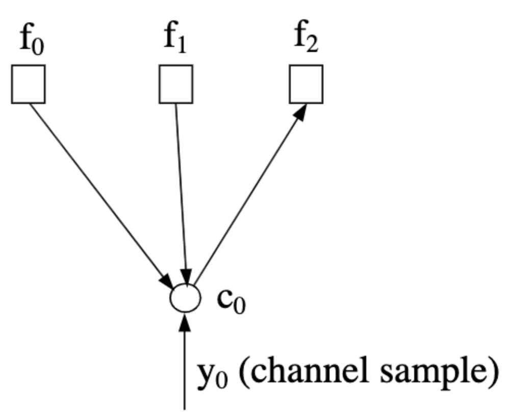
Message passing from variable to check nodes is referred to as passing up (denoted $m_{\uparrow ij}$). The information passed considers the probability $\Pr(c_i=b\vert \text{input messages})$. Assuming a Tanner graph corresponding to an $H$ whose zeroth column is $\left[1,1,1,0,\dots,0\right]^T$, the message $m_{\uparrow 02}$ is shown below. Note the direction of the arrows, which indicate the inputs used by node $c_0$ to formulate the message.
 |
|---|
| Image taken from An Introduction to LDPC Codes |
Passing Down
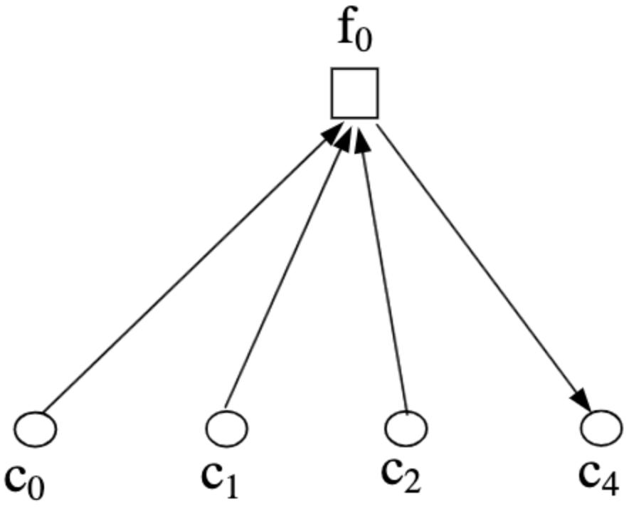
Message passing from check to variable nodes is referred to as passing down (denoted $m_{\downarrow ji}$). The information passed considers the probability $\Pr(f_j\text{ is satisfied}\vert \text{input messages})$. Assuming a Tanner graph corresponding to an $H$ whose zeroth row is $\left[1,1,1,0,1,,0\dots,0\right]^T$, the message $m_{\downarrow 04}$ is shown below. Note the direction of the arrows, which indicate the inputs used by node $f_0$ to formulate the message.
 |
|---|
| Image taken from An Introduction to LDPC Codes |
Algorithm Concept
The algorithm goes along the following lines:
- Each iterative step is divided into two half steps:
- First, all variable nodes pass messages to check nodes.
- Then, all check nodes pass messages to variable nodes.
- Iterations are done until a stop criterion or a predetermined threshold.
- After iterations are done, bit values $c_i$ are estimated to form a decoding decision.
The algorithm assumes messages are statistically independent. This assumption doesn’t hold if channel samples $y_i$ aren’t independent (which is possible). Even if samples are independent, the messages aren’t if the graph contains cycles (for girth $\gamma$, independence holds for $\gamma/2$ iterations). Nonetheless, even though the assumptions aren’t adhered to, simulations show the performance can still be good if short cycles are avoided.