Log Domain SPA
This page describes the sum-product algorithm in the log-likelihood domain
Outline of this page:
- Motivation
- Definitions
- Channel models
- Update rules
- Outlining the algorithm
- Discussion
Motivation
The probability domain version of the algorithm involves many multiplications. These multiplications may be costly in terms of computation for hardware implementation. It may also introduce numerical instabilities (multiplication by zero). As such, a version that involves additions is preferred.
Definitions
Define log-likelihood ratios (LLR):
- $L(c_i )=\log\left(\frac{\Pr(c_i=0\vert y_i )}{Pr(c_i=1\vert y_i ) }\right)$ - log-likelihood of bit values given channel symbols.
- $L(r_{ji}) = \log\left(\frac{r_{ji}(0)}{r_{ji}(1)}\right)$ - log-likelihood of validity of parity equation $j$ given bit value using information extrinsic to v-node $i$
- $L(q_{ij}) = \log\left(\frac{q_{ij}(0)}{q_{ij}(1)}\right)$ - log-likelihood of bit value (v-node $i$) using information extrinsic to c-node $j$.
- $L(Q_i)=\log\left(\frac{Q_i(0)}{Q_i(1)}\right)$ - log-likelihood of bit value (v-node $i$).
For the LLR version of the algorithm, the messages passed are:
\[m_{\uparrow ij}=L(q_{ij})\]and
\[m_{\downarrow ji}=L(r_{ji} )\]Channel Models
The channel dependency is also transformed to log domain.
- BEC – channel samples are $y_i\in\{0,1,E\}$, for which:
- BSC – with error probability $\epsilon$, channel samples are $y_i\in\{0,1\}$, for which:
- BI-AWGNC (binary input AWGN channel). Channel inputs are $x_i=1-2c_i$, and channel samples are $y_i=x_i+n$, where $n\sim N(0,\sigma^2 )$, for which:
Update Rules
Following An Introduction to LDPC Codes (p.13-14), we get the following update rules:
- $L(r_{ji})$ - Define $L(q_{ij})=\alpha_{ij} \beta_{ij}$, where $\alpha_{ij}=sign(L(q_{ij}))$, and $\beta_{ij}=\vert L(q_{ij})\vert$. The sign may be thought of as bit value, while magnitude corresponds to reliability. Then:
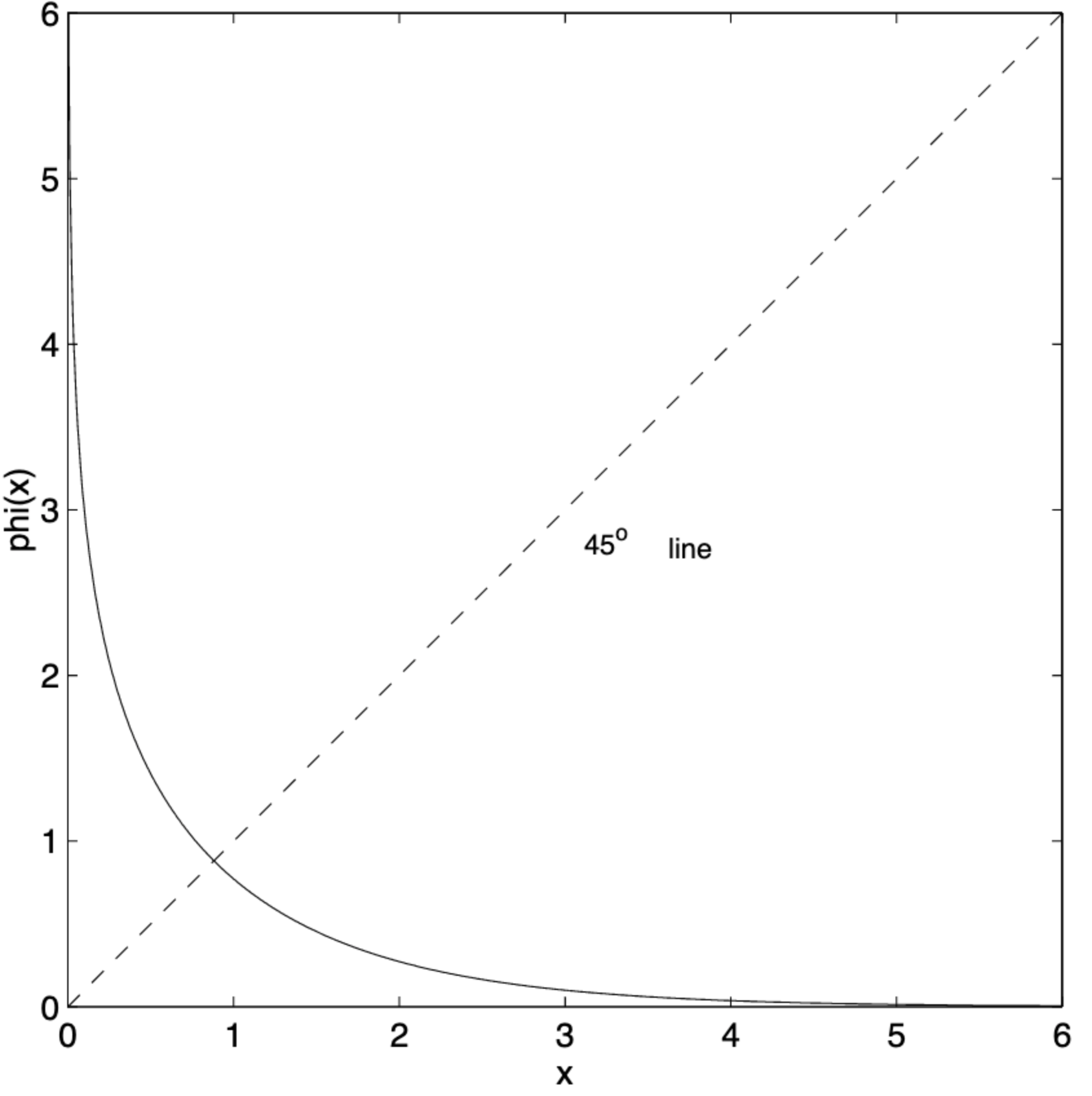
where: $\phi(x)=-\log{\left[\tanh{\left(\frac{x}{2}\right)}\right]}=\log{\left(\frac{e^x+1}{e^x-1}\right)}$
- $L(q_{ij})$ - Using the above, we may do:
- $L(Q_i)$ - Similarly we may do:
Algorithm
- For $n$ bits initialize: $L(q_{ij})=L(c_i )$, for all $i,j$ for which $h_{ij}=1$
- Update $L(r_{ji})$
- Update $L(q_{ij})$
- Update $L(Q_i )$
- For all $n$ bits decode \(\hat{c}_i=\begin{cases}1 & L(Q_i)<0\\ 0 & \text{else}\end{cases}\)
- If $H\hat{c}^T=0$ or exceeded maximal iterations limit, stop, else go to step 2.
Discussion
- The complicated function $\phi(x)$ is relatively well-behaved for $x>0$ (see figure below) and can be implemented using a lookup table.
- Reduced complexity versions of this decoder exist where the product can be eliminated subject to some approximations.
 |
|---|
| Image taken from An Introduction to LDPC Codes |