Representation

This page describes various representations of LDPC codes

---

Matrix Representation

Generator and parity check based representation

As with all linear codes, every codeword $c\in C$ of an $(n,k)$ code belongs to a $k$ dimensional linear subspace of $F^n$. As such, a base for the subspace may be found, and every codeword may be expressed using a generator matrix via: $c=uG$, where $u\in F^k$ is some vector holding information, and $G$ is a matrix whose rows are the base of the subspace.

The $(n-k)$ dimensional null space of $G$, whose vectors adhere to $xG=0$, also has a base. The parity check matrix $H$ rows are made of these base vectors (the choice isn’t unique). In turn, each row of the $(n-k)$ rows of $H$ defines a specific parity check equation as for every legitimate codeword $c\in C$, we have $Hc^T=0$, which is yet another way to express the set of all codewords.

Weights

A low density parity check code is defined via a sparse matrix $H$. For a regular LDPC code the weight (number of nonzero values) of each column is the same and equal to some $w_c$, while the weight of each row is $w_r= w_c\left(\frac{n}{m}\right)$. Typically, $H$ is of full rank which implies $n-k=m$, in which case the rate of the code depends on the wights via $R=\frac{k}{n}=1-\frac{w_c}{w_r}$.

---

Graph Representation

Tanner Graph

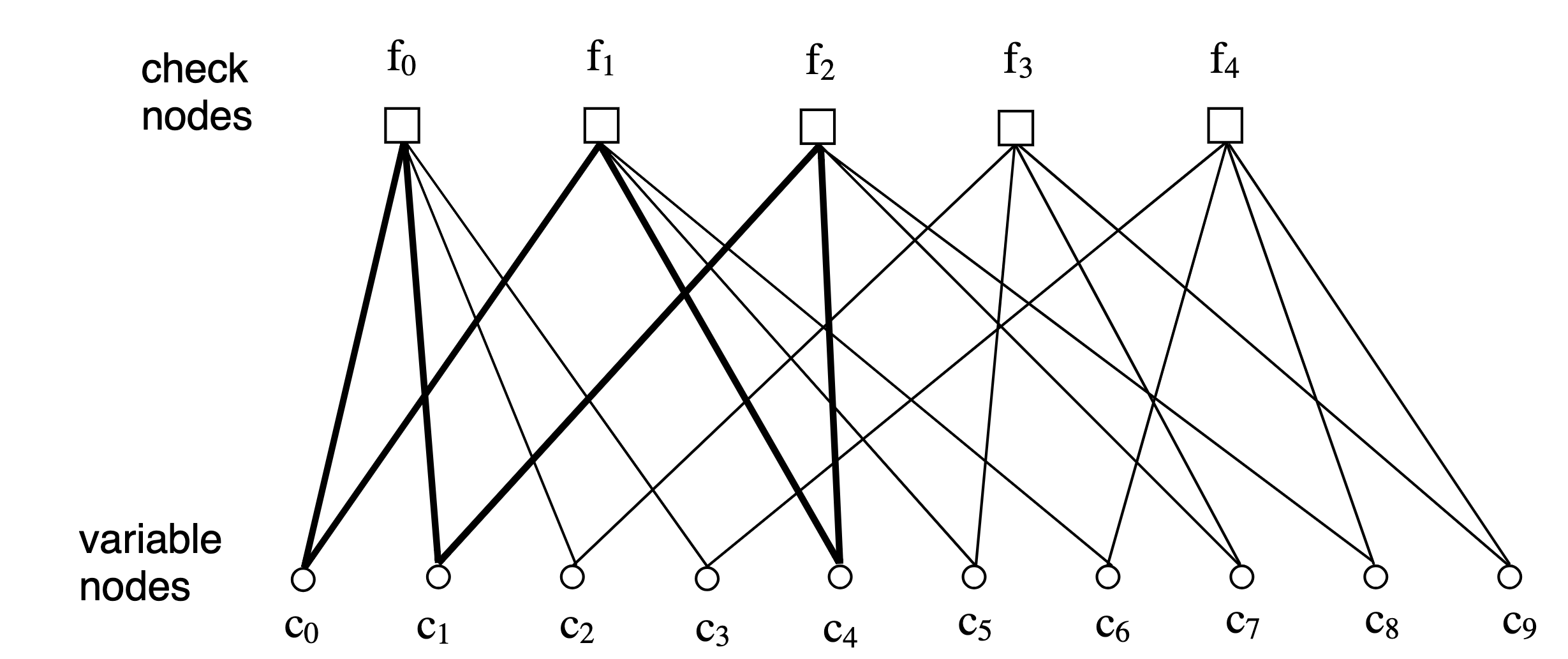
The following discussion regards only codes over binary alphabets. For such codes, the parity check matrix can be expressed using a bipartite graph called a Tanner graph (after Tanner, who invented them). The two families of nodes are called variable nodes (denoted in below graph as $c_i$) and check nodes (denoted in below graph as $f_i$). For an $(n,k)$ code there are $m=n-k$ check nodes (one per parity check equation), and $n$ variable nodes (one per information bit in codeword). The parity check matrix $H$ dictates the graph via the following rule: check node $j$ is connected to variable node $i$ when $h_{ji}=1$. As an example the $(10,5)$ code specified by:

\[H = \begin{bmatrix} 1 & 1 & 1 & 1 & 0 & 0 & 0 & 0 & 0 & 0 \\ 1 & 0 & 0 & 0 & 1 & 1 & 1 & 0 & 0 & 0 \\ 0 & 1 & 0 & 0 & 1 & 0 & 0 & 1 & 1 & 0 \\ 0 & 0 & 1 & 0 & 0 & 1 & 0 & 1 & 0 & 1 \\ 0 & 0 & 0 & 1 & 0 & 0 & 1 & 0 & 1 & 1 \\ \end{bmatrix}.\]

Per the rule, the matrix corresponds to the graph:

Image taken from An Introduction to LDPC Codes

For instance, $f_0$ is connected to $c_0,c_1,c_2,c_3$ as implied by the first row of $H$. Since this code is regular, every variable node has two edges, and each check node has four edges. A Tanner graph is characterized by a cycle and a girth. A cycle of length $\nu$ in a Tanner graph is a closed path of $\nu$ edges. The bold edges exhibit a cycle of 6 edges in the example graph shown above. A girth $\gamma$ of a Tanner graph is the minimum cycle length in the graph. Short cycles degrade the decoding performance of an LDPC decoder.