Probability Domain SPA
This page describes the sum-product algorithm in the probability domain
Outline of this page:
- Definitions
- Factorization of complicated expressions into simpler ones
- Discussion of channel models and how they come into play in LDPC codes
- Outlining the algorithm
- Discussion
Definitions
We begin with a set of definitions:
- $V_j$ - set of v-nodes connected to c-node $f_j$.
- $V_j/i$ - set of v-nodes connected to c-node $f_j$, except v-node $c_i$.
- $C_i$ - set of c-nodes connected to v-node $c_j$.
- $C_i/j$ - set of c-nodes connected to v-node $c_i$, except c-node $f_j$.
- $M_v (\sim i)$ - set of messages from all v-nodes except node $c_i$.
- $M_c (\sim j)$ - set of messages from all c-nodes except node $f_j$.
- $P_i=\Pr(c_i=1\vert y_i )$, where $y_i$ is the channel input (channel model dependent).
- $S_i$ - the event that parity check equations involving node $c_i$ are satisfied.
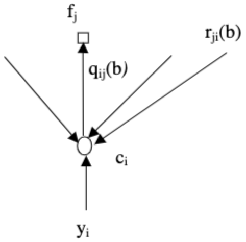
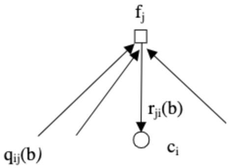
- $q_{ij} (b)=\Pr(c_i=b\vert S_i,y_i,M_c(\sim j))$ - with $b\in\{0,1\}$. For probability domain algorithm we get $m_{\uparrow ij}=q_ij (b)$.
- $r_{ji}(b)=\Pr(\text{check equation } f_j \text{ is satisfied}\vert c_i=b,M_v (\sim i))$ - with $b\in\{0,1\}$. For probability domain algorithm we get $m_{\downarrow ji}=r_{ji}(b)$.
Note that the listed probabilities are, in fact, random variables as they are functions of the random channel samples $y_i$. As shown in the figure below, for the probability domain algorithm, $q_{ij}$ are the messages passed from v-nodes to c-nodes, while $r_{ji}$ are the messages passed from c-nodes to v-nodes.
 |  |
|---|---|
| Image taken from An Introduction to LDPC Codes |
Factorizing $q_{ij}(b)$
Due Bayes rule and assumed independence we may factorize (see An Introduction to LDPC Codes for details):
\[q_{ij} (0)=\Pr(c_i=0\vert S_i,y_i,M_c (\sim j))=K_{ij} (1-P_i)\prod_{j'\in c_i/j}r_{j'i} (0)\]and similarly:
\[q_{ij} (1)=K_{ij}P_i\prod_{j'\in c_i/j}r_{j'i} (1)\]where $K_{ij}$ are chosen such that $q_{ij}(0) + q_{ij}(1) = 1$. Note that the products involve all check nodes $j’$ which have edges connecting to variable node $i$, except for check node $j$, as required previously when we dictated that the algorithm passes only extrinsic information.
Factorizing $r_{ji}(b)$
Note the following observation made by Gallager. Consider a sequence of $M$ independent bits $a_i$, for which $\Pr(a_i=1)=p_i$. Then the probability of having an even number of 1’s is:
\[\frac{1}{2}+\frac{1}{2}\prod_{i=1}^M (1-2p_i )\]which can be found by induction on $M$. Now, for equation $f_j$ over a binary alphabet, to satisfy the parity check requirement, it must contain an even number of 1’s. Thus, by mapping $p_i\to q_{ij}(1)$ and conditioning on $c_i=0$ (so that all other bits must have an even number of 1’s), we get from the definition:
\[r_{ji}(0) = \frac{1}{2}+\frac{1}{2}\prod_ {i'\in V_j/i}(1-2q_{i'j}(1))\]By normalization:
\[r_{ji}(1) = 1- r_{ji}(0)\]Channel Models
So far, the derivation was channel-independent. However, the messages depend on $P_i=\Pr(c_i=1\vert y_i )$ which is clearly channel dependent. As an example, we consider three channels:
- BEC – channel samples are $y_i\in\{0,1,E\}$, for which:
- BSC – with error probability $\epsilon$, channel samples are $y_i\in\{0,1\}$, for which:
- BI-AWGNC (binary input AWGN channel). Channel inputs are $x_i=1-2c_i$, and channel samples are $y_i=x_i+n$, where $n\sim N(0,\sigma^2 )$, for which:
Algorithm
- For $n$ bits set $P_i=\Pr(c_i=1\vert y_i )$, then initialize: $q_{ij}(0)=1-P_i$ and $q_{ij}(1)=P_i$, for all $i,j$ for which $h_{ij}=1$.
- Update $r_{ji}(b)$ using $q_{ij}(b)$.
- Update $q_{ij}(b)$ using $r_{ji}(b)$, and normalize by setting $K_{ij}$.
- For all $n$ bits compute the following: $Q_i (1)=K_i P_i \prod_{j\in C_i}r_{ji} (1)$, and $Q_i (0)=K_i (1-P_i ) \prod_{j\in C_i}r_{ji}(1)$. Note that no nodes are omitted here. Set $K_i$ such that $Q_i (1)+Q_i (0)=1$.
- For all $n$ bits decode \(\hat{c}_i=\begin{cases}1 & Q_i(1)>Q_i(0)\\0 & \text{else}\end{cases}\)
- If $H\hat{c}^T=0$ or exceeded maximal iterations limit, stop, else go to step 2.
Discussion
- The presented algorithm may be optimized prior to implementation, For instance step 4 may precede step 3, and then step 3 may be replaced with $q_{ij}(b)=K_{ij}Q_i(b)/r_{ji}(b)$.
- This version is intuitive and has an intuitive interpretation regarding the estimated quantity. However, it involves numerous multiplications, which are computationally expensive. The log-based version allows substituting multiplications by sums.